Pulsar Observation
Introduction
The challenge begun during the 2014 summer in company with my
friend IW1DTU.
The inspiration was taken from the results
achieved by Joe K5SO and well described in his web site: K5SO
Radio Astronomy
The choosen target was the PSR B0329 + 54
which is the brightest radio pulsar visible in the northern sky
The
pulsar is 2643 light-years away from solar system and completes one
rotation every 0.71452 seconds and is approximately 5.5 million years
old.
A pulsar is a rotating neutron star that emits a beam of
wide spectrum of electromagnetic radiation. Being the peak of
radiation around 380Mhz the closer amateur band was the 70cm and
hence we decided to use my 16 x 26 array with the 70cm receiver
chain.
Difficulties
The detection of a pulsar signal is certainly a big challenge for
an amateur installation because signals are very weak. It is possible
for amateur radio astronomers to detect some of the stronger pulsars
by use of digital signal processing techniques given an adequate gain
antenna, it is therefore mandatory to use a modern SDR digital
receiver to be able to detect the faint pulsar signal.
One trick
to make things easier is to know in advance the pulsar period. In
that case the receiver samples can be combined together in sync with
the known pulsar period to enhance the coherent pulses and smooth the
background noise (data folding). Data folding consists in averaging
many block of received samples each with a time length corresponding
to the pulsar period, that implies a long period of observation
(hours). The pulsar is a wide spectrum transmitter and its signals
are detected by looking at the level variation of background noise
and inspecting it in the time domain. The amount of excess noise is
therefore depending on total noise received and examined it is then
important make the observation on a bandwidth as wide as we can(up to
a certain limit).
SetUp
The setup was composed by the following:
I1NDP Installation
70cm array with pulsar tracking capability
0.3db NF, 30db gain
LNA
70 cm Transverter
Rubidium disciplined signal generator
IW1DTU portable receiving station
Frequency divider (by 10000000)
SDR 14 connected to the
28Mhz IF output of the transverter
Sprectravue software
Personal
computer
Principles
The SDR14 SDR Receiver (RS Space) has provision for an
external signal triggering the collection of samples at specific
intervals. By setting properly the signal generator and going trough
the frequency divider it is possible to provide trigger pulses with
interval in accordance with the pulsar period.

Not all set yet because the signal that we are going to search
are unfortunately effected by doppler depending on the relative
motion of astral object and the location from where takes place the
observation. K5SO, which deserves our gratitude for his help and
useful suggestions, provided for us a version of the well known
"tempo" utility which could run on our PCS.
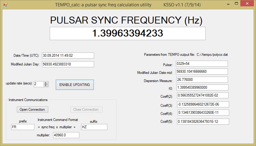
By giving the proper input parameters (astral object,local
position, current time) the given frequency value is used for a
correct setting of the signal generator. Other options of the SDR14
receiver are tailored for radio astronomy and particularly the
capability of data folding and graphic representation in the time
domain.
70cm Pulsar Observation
We made several attempts in more than one occasion but ,very
disappointed, we were not able to identify any sign of the pulsar.
Unfortunately the 432Mhz band in my location is suffering of a very
high degree of RF pollution and the background noise is always very
high. When i first built the antenna the sun noise measurement was
giving an excess of 17db as Y factor (cold sky vs sun) while i am
currently getting something between 15 to 16db at best. In addition
the array needs some deep cleaning of the feed line joints which at
time become noise generators when antenna moves.
We hoped that
the data folding process could cope with the high level of noise but
it was not the case. We understood we had to try a different
approach.
23cm Pulsar Observation
The decision was to try on 23cm which is a much quieter
frequency using my 10m dish, on 23cm the weaker pulsar can (hardly)
be compensated by the higher antenna gain and actually the attempt we
made with the same setup as on 70cm (SDR 14 + Hardware trigger) and
about 2 hours of observation have also been disappointing. No sign of
the pulsar. The only chance of increasing our sensitivity was to
enlarge the bandwidth window but the SDR14 is not able to go beyond
the 250Khz limit.
I own a Perseus SDR with a typical mission as
an excellent HF receiver but no provision as radioastronomical tool
but it is capable of producing a 2Mhz wide spectrum recording as a
.wav file. The chance was to try with an off line data integration
produced by the Perseus using an ad hoc home made software.
The
receiving chain was then composed by 10mdish + 0.27db NF, 37db gain
LNA + transverter + Perseus at 28Mhz IF, the feeder was a septum dual mode with circular polarization.
The software was composed by
a processing task reading the .wav file and integrating all of the
recorded samples in a memory table and a raw graphic object to show
the final result. Input to the processing was the pulsar frequency
calculated by the TEMPO utility for current frequency,location and
time. Next essential information was the sample rate use by the
receiver and it was taken from the .wav header information.
23cm Integration Process
The integration process consist in keep adding blocks of
samples corresponding to an integer number of pulsar period (data
folding) producing at the end a mean value for each sample in such a
way to enhance coherent signals and weaken the random noise.
The
longer the period covered by the recorded file the better the chance
of making the feeble signal to show up. At the end of each cycle of
data folding a common value corresponding to the lower recorded mean
was subtracted to each table position.
The .wav file is a 2
channel interleaved recording, the I & Q samples are used to
calculate the magnitude of the vector which is then integrated.
23cm Pulsar Observation Results
The first results were not very encouraging until we decided
to try changing the sample rate and making it a variable input
parameter. The Perseus is driven by a quartz oscillator and, as any
equivalent oscillator, prone to suffer of frequency variation due to
several factors so we could not rely on what stated in the .wav file.
As input parameter is foreseen also the definition of the time
window of observation in an integer number of pulsar period as well
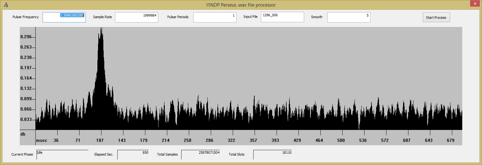
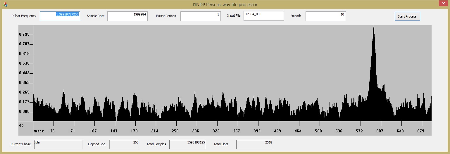
as a smoothing parameter. After several attempts finally we started
to see signs of the pulsar. The followings are a few screen shots
produced by our own graphic output object from the same file but at
different time length.
The total observation time was more than 3
hours for a total of 96.4 Gbytes of collected samples.
The x
scale in milliseconds shows the distance in time between different
pulses corresponding to the pulsar period (0.714sec)
On the Y axe
the db scale has as reference the level of noise floor at the end of
the integration and gives a flavor of how weak is the received
signal.
1 Period
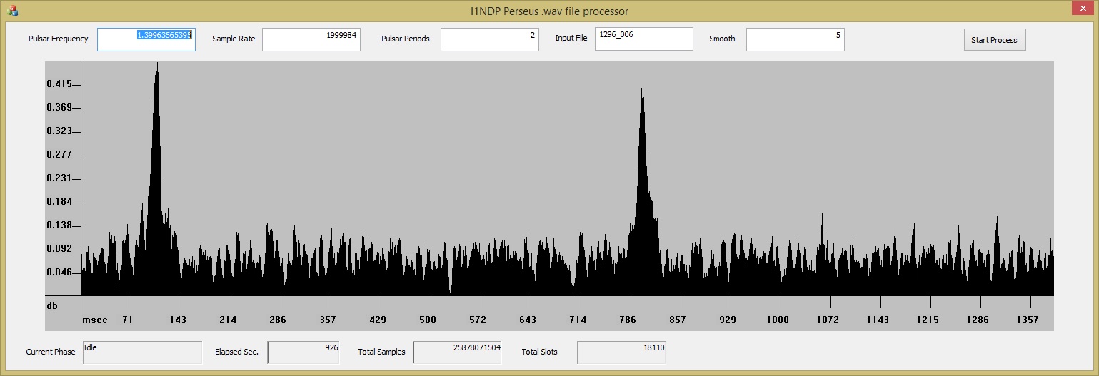
2 Periods
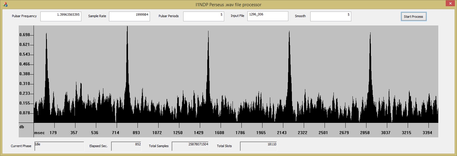
5 Periods
23cm Pulsar Observation Validation
All of the above have been the results of a single
observation, i needed to verify the result as not being produced by
accident. The first trial was to make a long oservation with the
antenna pointing on cold sky so completely off target. Several
attempts to tune sample per seconds parameter did not produce other
then noise as result of data analysis. Next was one hour recording
(on target this time) and then serach for the pulsar signal, it came
out but with a low S/N ratio and therefore not a satisfactory result.
A light rain during the observation period could justify the poor
outcome. Finally with a 3 hours recording i was able to see again
well defined shapes of the pulsar signal and actually the star came
out of noise after only a few minutes of recorded data. The following
are the graph produced by the observation cut to only about 1800sec
because a longer processing was worsening the S/N ratio. The reason
was the low elevation of B0329 + 54 and the dish was starting to pick
up groound noise
1 Period
Pulsar Data Processing
The following link runs a flash movie showing the coming out of
the pulsar signals on graph from the back ground noise during the off
line data processing:
 Data Processing
The time window was set to 3 pulsar
periods. The input files are those recorded with the Perseus receiver
during the last observation.
The duration of the movie
corrensponds to the real processing time (including the long file
reading from disk).
The time of observation is of 2517 pulsar
periods or 1800 seconds.
K1JT Suggestions
I received the best, by far, confirmations off my efforts from Joe
Taylor (Nobel prize on a pulsar study) which i involved in my
activity with a simple question but he was interested in what i did.
Once i sent him a copy of my recordings i received the following
feedback as a graph:
K1JT Analysis 1
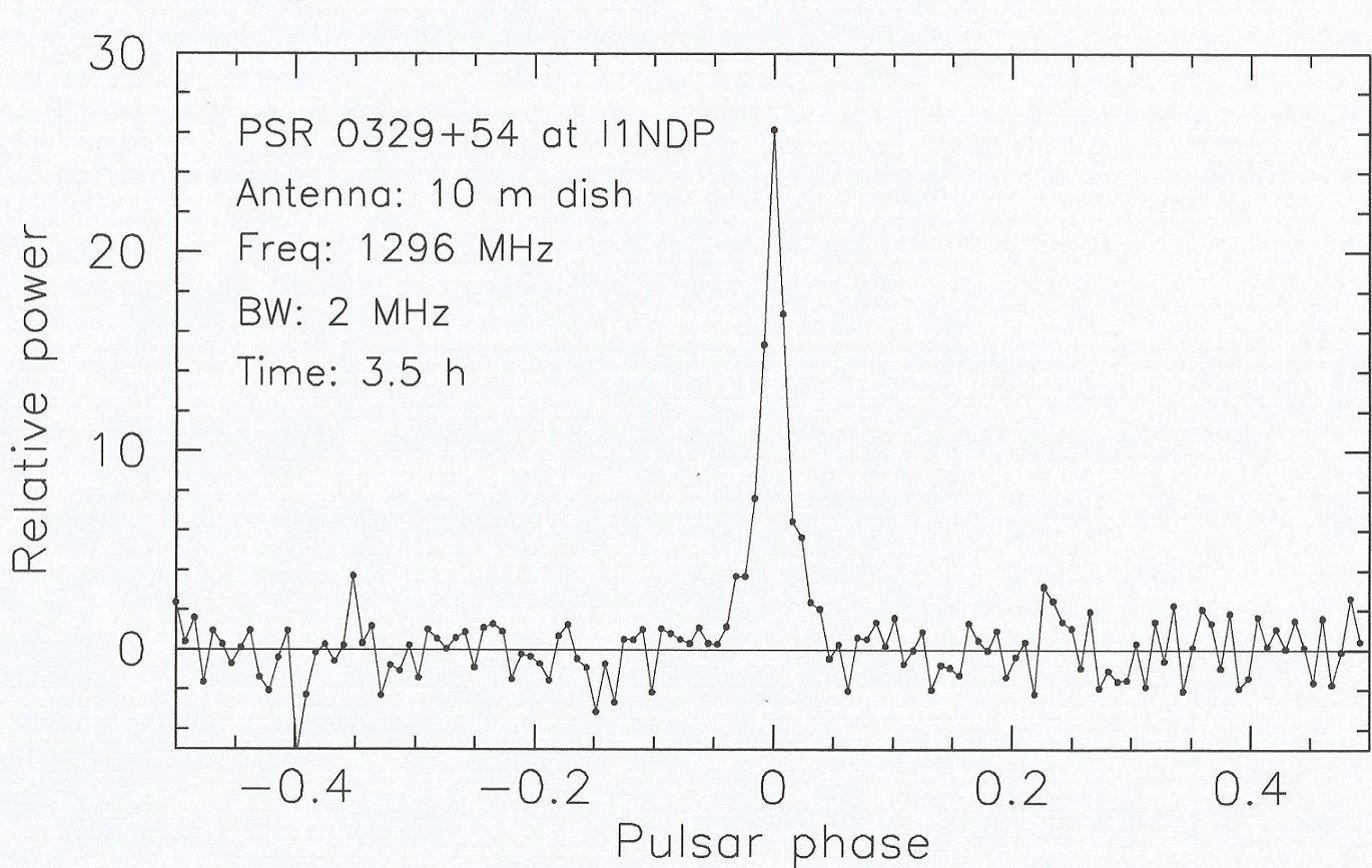
And that was his comment:
"I folded the
data into 128 equally spaced phase bins covering the full pulsar
period, obtaining the average pulse profile shown in the attached
plot.
Pulsar phase is shown in units of periods; the pulse was
arbitrarily rotated to put the peak at phase zero, in the middle.
The average off-pulse noise power was measured and subtracted,
and the power was scaled so that the rms noise on the plotted
baseline is 1.0.
Thus, at the resolution indicated the observed
signal-to-noise ratio is about 26. It's a beautiful set of
observations!"
But is not all, i received also some
suggestions on what could be done in a better way.
1) It is
not necessary to process the whole bunch of samples for long period
observations.
The original recording can be decimated to produce
smaller amount of data easier to handle without loosing information
as long as the final definition is a small percentage of the pulsar
period.
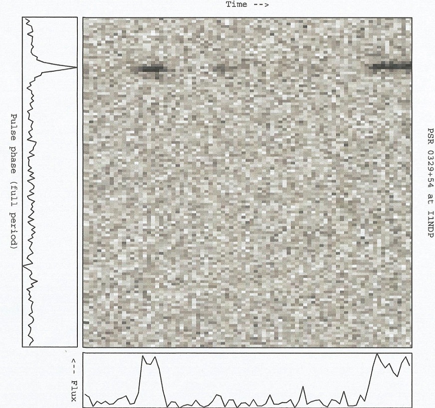
2) The pulsar signal is not constant and can have deep fading due
to the effects of interstellar scintillation so being able to select
only portions of the observation period is theoretically possible to
achieve a better definition of the pulsar shape.
To show the
meaning of the above he provided me with the following graph:
K1JT Analysis 2
The vertical axis is pulse phase (one full period) and the
horizontal axis is time (0 to 3.5 hours).
3) An off line processing should be preferred to any real
time observation.
Pulsar software revision
Following the above indications i tried to modify my data
processing code by building something more structured and with some
flexibility.
Software root
The application, in order to an easy handling of huge files, is
compiled for a 64 bits window system (I use W8).
Made as a pop up
screen allows the selection of a few functionalities:

Decimate
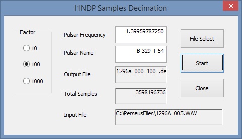
The required input are the value of the pulsar frequency at
the moment of observation, the decimation ratio, the first of the
.wav files to be decimated and a title.
The output consist of a
single .dec file made of a header with relevant information on
original file set and an array of "float" values
representing the I+Q samples as averaged power value.
Integrate
It does not have an interface but allows the selection among
the available.dec files to be integrated in memory according with the
selected pulsar number of periods.
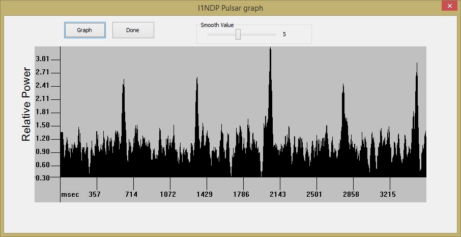
Graph
Produces a solid graph using the integrated data available in
memory in the same fashion as the previous graphs. The following is
produced by an integration of 5 periods of the half an hour
observation.
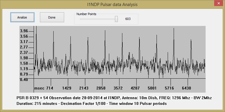
Analyze
A different fashion in graphics with some additional
information on the origin.
The following is produced by an
integration of 10 periods.
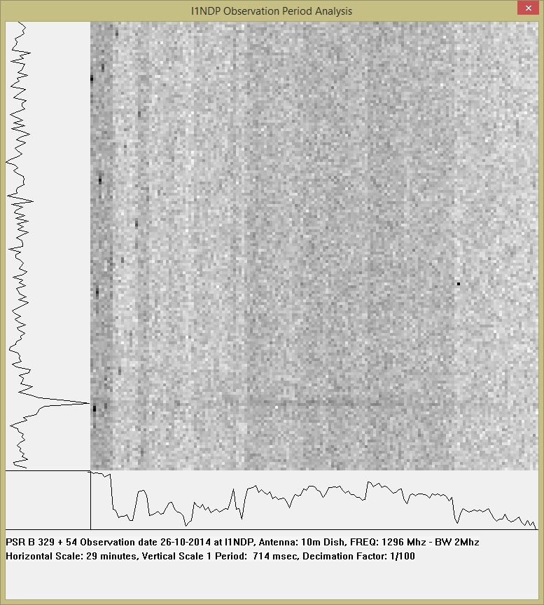
Observation Check
This is an attempt of doing the same analysis suggested by Joe
but not sure if bug free yet!
This should be the analysys of
the lucky observation half an hour long where the feeble pulsar track
is visible for the whole duration and hence a well defined pulsar
phase output.
Nevertheless i have to say that i tried ,based on Joe
analysis, to select which periods to integrate and which to discard
but the output quality did not improve.
At the contrary, spikes
of noise which were easily absorbed by a long period of integration
were still visible at the end.
What's next?
I made several attempts with other possible targets but so far
the only success was the detection of PSR B1933 + 16 with a weaker
signal compared to B0329 + 54.
Unfortunately by mistake i deleted
all the files. Only one screen shot left:
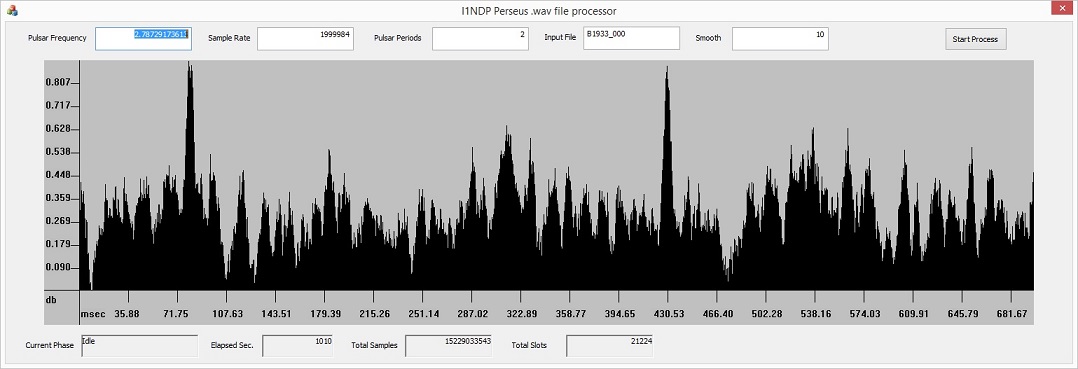
The neutron star makes almost 3 revolutions per second and
the distance to 1933+16 is estimated to be about 26000 light years.
I hope to be able to make a better observation of this star in
the future.
A couple of recording from B 0531 + 21 (crab
pulsar) and B1822-09 were attempted but no results.
The crab
pulsar, althougth is producing very strong signals (giant pulses), is
very difficult to detect because they are not predictable and
interleave with much weaker ones.
B 1822 - 09 instead has a low
declination and, i suspect, that the ground noise picked up by the
antenna will preclude its detection.